Bayesian Sensor Calibration: A Pythonic Approach
As a sensor engineer, I’ve always been fascinated by the intricacies of sensor calibration. The process of optimizing sensor performance is crucial in various industries, from healthcare to aerospace. In this article, I’ll delve into the world of Bayesian sensor calibration, exploring its applications and benefits using Python.
The Importance of Sensor Calibration
Physical sensors are the primary inputs that enable systems to make sense of their environment. However, sensors are never perfect, and non-idealities, part-to-part variations, and random noise contribute to sensor error. Calibration and subsequent adjustment are critical steps to minimize sensor measurement uncertainty. The Bayesian approach provides a mathematical framework to represent uncertainty.
A Simplified Case Study
Let’s consider a magnetic field sensor whose sensitivity drifts with temperature. We’ll use a Bayesian approach to calculate the optimum set of calibration parameters for a given calibration dataset. This approach provides a trade-off between the classic full regression and blind calibration methods.
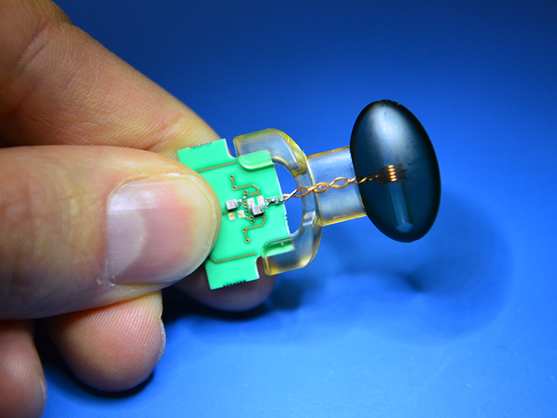 Magnetic field sensor
Mathematical Formulation
We assume that the magnetic sensor consists of a magnetic and temperature transducer, which can be modeled as polynomial transfer functions with coefficients varying from one sensor to the next according to normal probability distributions.
Python Formulation
We use the code convention introduced by Close (2021). We define a data dictionary dd to store the nominal value of the parameters. In addition, we define the probability density functions capturing the variability of the parameters.
Classic Approaches
We first consider two well-known classic calibration approaches that don’t rely on the Bayesian framework: full regression and blind calibration.
Full Regression
The first calibration approach is a brute-force approach. A comprehensive dataset is collected for each sensor, with more calibration points than unknowns. The calibration parameters w for each sensor (4 unknowns) are determined by a regression fit.
Blind Calibration
A blind calibration represents the other extreme. In this approach, a first reference set of sensors is fully calibrated as above. The following sensors are not individually calibrated. Instead, the average calibration parameters w0 of the reference set is reused blindly.
Bayesian Calibration
The Bayesian calibration is an interesting trade-off between the previous two extremes. A reference set of sensors is fully calibrated as above. The calibration parameters for this reference set constitute some prior knowledge. The average w0 and the covariance matrix Σ encode some relevant knowledge about the sensor response.
Conclusion
In this article, we presented a Python workflow for simulating Bayesian sensor calibration and compared it against well-known classic approaches. The mathematical and Python formulations are valid for a wide class of sensors, enabling sensor design to explore various approaches.
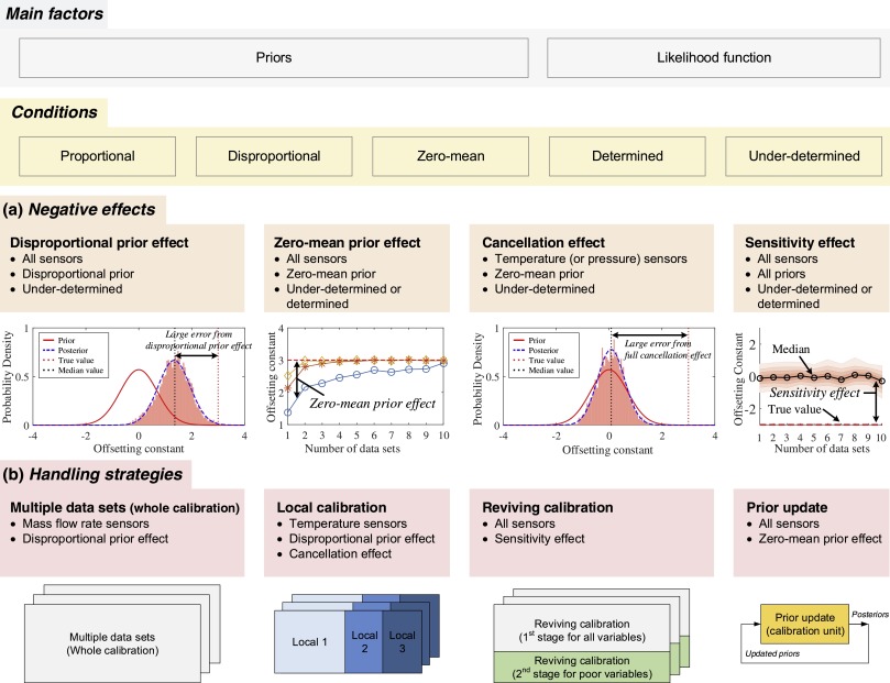 Bayesian sensor calibration
References
- Berger, M., Schott, C., & Paul, O. (2022). Bayesian sensor calibration. IEEE Sens. J.
- Close, G. (2021). Signal chain analysis in Python: a case study for hardware engineers. Towards Data Science.
- Copley, C. (2023). Navigating Bayesian Analysis with PyMC. Towards Data Science.
- Davidson-Pilon, C. (2015). Bayesian Methods for Hackers: Probabilistic Programming and Bayesian Inference. Addison-Wesley Professional.
- Martin, O. A., Kumar, R., & Lao, J. (2021). Bayesian Modeling and Computation in Python. Chapman and Hall/CRC.
- Watts, A. (2020). PyMC3 and Bayesian inference for Parameter Uncertainty Quantification Towards Non-Linear Models: Part 2. Towards Data Science.


